Conditional Formatting

Conditional formatting allows you to visually highlight and analyze your data by applying specific rules. You can enhance data analysis with the conditional formatting feature for tables and pivot tables. This powerful tool allows you to define custom rules to dynamically color-code cells based on their values. It provides a strong reasoning for its use by enabling quick visual identification of key data points that meet specific thresholds or criteria, which is a far more efficient method of data comprehension than manual inspection.

Note

• The conditional formatting capability is exclusively available for Table and Pivot table widgets.
• Conditional formatting can be done for numeric columns as well as for text columns. For example, for a Payment type column, you can add conditions to add blue color to all payments done using Credit Card.

The key features of conditional formatting in DataGOL includes:

• Multiple conditions per column: You can apply several conditional formatting rules to a single column, allowing for nuanced visual analysis and detailed segmentation of your data. You can define multiple rules for your data based on two main types of values:

  • Thresholds: Set rules based on whether a value is greater than, less than, greater than or equal to, or less than or equal to a specific number. For example, you could color all values over 10,000,000 green to quickly identify top performers.

  • Ranges: Define a spectrum of colors for values that fall within a specified minimum and maximum. This creates a gradient effect, such as shading values between 5,000 and 10,000 in a gradient of yellow, which helps in understanding the distribution of data.

    For instance, you could highlight revenue cells in green if they exceed $10,000, yellow if they fall between $5,000 and $10,000, and red if they are below $5,000.

  Note

  • If multiple rules are created, the first rule takes preference over the second. The system checks the first rule, and if it is a match, it is applied, and the other rules are ignored. f the first rule does not match, the system moves on to the second rule.
  • You can change the priority of the rules by moving them up or down.

• Data Bars: These rules add a bar inside each cell to visually represent its value relative to other values in the column.

• Column Comparison: Column comparison is a conditional formatting feature that allows you to compare values in one column to another. It's a more dynamic and advanced option than a standard value comparison, which only compares a column's values against a fixed value.

• Customize formatting styles: Choose to alter the text color and/or the background color of the cells to effectively draw attention to specific data points. You can now define custom rules and dynamically color-code cells based on their values, allowing for quick visual identification of key data points that meet specific thresholds or criteria.

  For example, you can highlight revenue cells in green if they exceed $10,000, yellow if they fall between $5,000 and $10,000, and red if they are below $5,000.

How to set rules for conditional formatting?

To apply conditional formatting, you need to set up rules that will highlight specific data in your tables.

1. From a workspace, navigate to the visualizer and generate a Table or Pivot table widget. From a table or pivot table, you can create new rules and manage existing ones.

2. From the right panel, click Update Widget Column Configurationsicon and click the column where you want to apply the conditions or rules.

3. From the slide-out menu, in the Conditional Formatting section, click Add Rules button. The Conditions Formatting Rules pane is displayed.

4. Click Conditions. The Conditions Formatting Rules dialog box is displayed with Rule type auto-selected as Conditions. Do the following:

   • Select the logic: AND condition or the OR condition.

   • Choose a Comparison Type: You have two options for your comparison:

     • Value Comparison: Compare the column's value against a static, fixed value (e.g., is greater than 500). You can compare using the following operands:

       • Greater Than
       • Less Than
       • Equal To
       • Not Equal To
       • Greater Than or Equal To
       • Less Than or Equal To
       • Between
       • Is Null
       • Is Not Null
       • In
       • Not In

     • Column Comparison: Lets you compare the column's value against the value of another column in your report. For this to work, you can only compare metric columns with other metric columns, and dimension columns with other dimension columns. You can compare using the following operands:

       • Equal To
       • Not Equal To
       • Contains
       • Not Contains
       • Starts With
       • Ends With

   • Set complex rules (Optional):** You can combine multiple conditions using AND or OR logic. This allows you to create more sophisticated rules, such as "value is greater than 100 AND less than 200."

   • Define Formatting:** Choose the colors, font styles, and other visual options to apply to cells that meet your defined conditions.

5. Optionally, you can add more rules or set up data bars.

6. Click Apply and in the slide-out menu, click Apply. The conditional formatting gets applied with the conditions or rules set are met.

How to set up data bars in columns?

Data bars provide a quick, visual overview of values within a column without needing to read the numbers.

1. From a workspace, navigate to the visualizer and generate a Table or Pivot table widget. From a table or pivot table, you can create new rules and manage existing ones.

2. From the right panel, click Update Widget Column Configurationsicon and click the column where you want to apply the conditions or rules.

3. From the slide-out menu, in the Conditional Formatting section, click Add Rules button. The Conditions Formatting Rules pane is displayed.

4. Click Data Bar. The Conditions Formatting Rules dialog box is displayed with Rule type auto-selected as Data Bars.

5. Configure Settings: Data bars are based on the values within their specific column. You can customize the bar's appearance by adjusting:

   • Bar Direction & Axis: Set the direction of the bar and control the position of the axis within the bar.

     
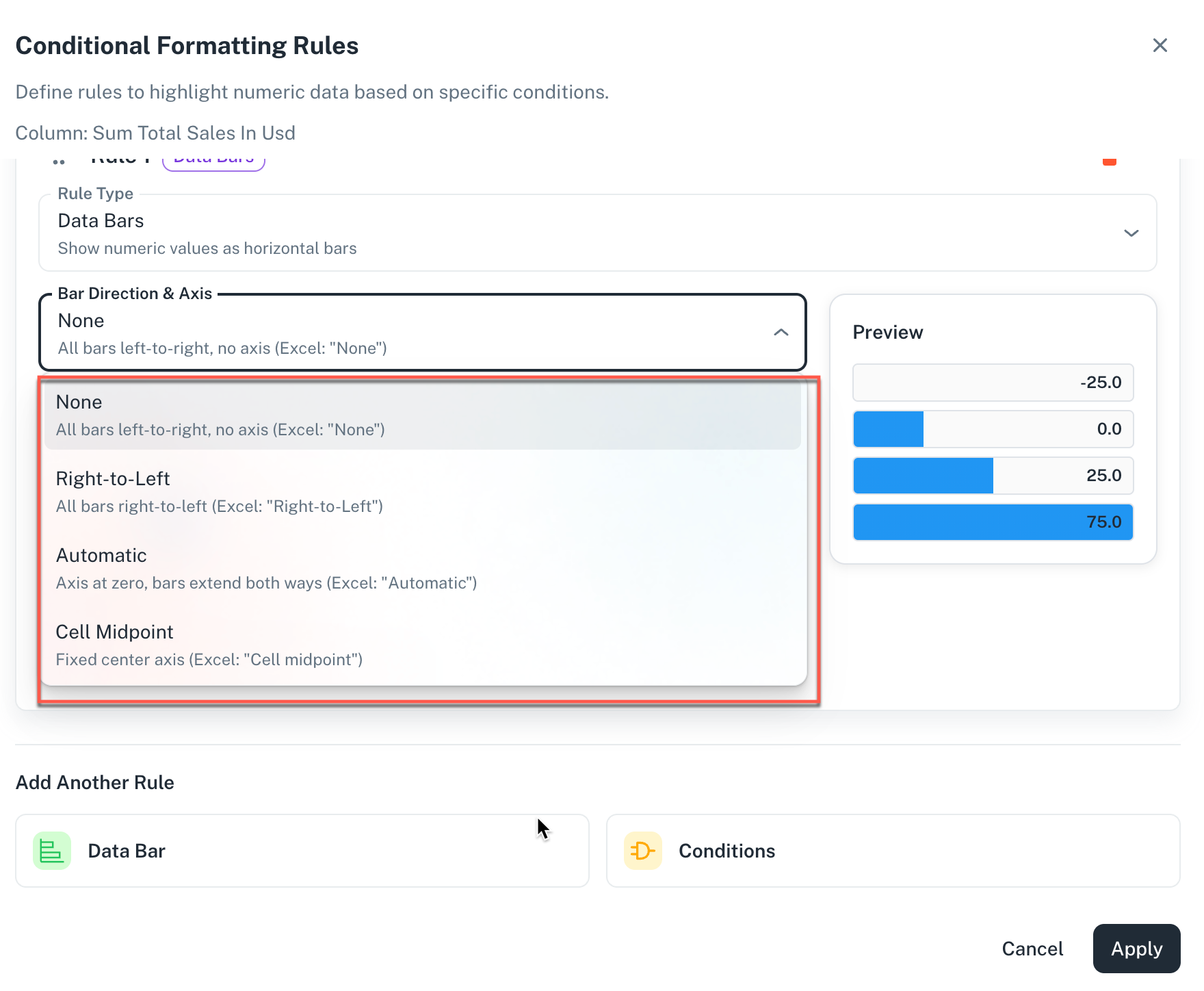
     • None: This option will set the bars from left to right without any axis.
     • Right-to-Left: This option will set the bars from right to left with right to left axis.
     • Automatic: The bars can extend in both ways while the axis is at zero.
     • Cell Midpoint: Fixed center axis.

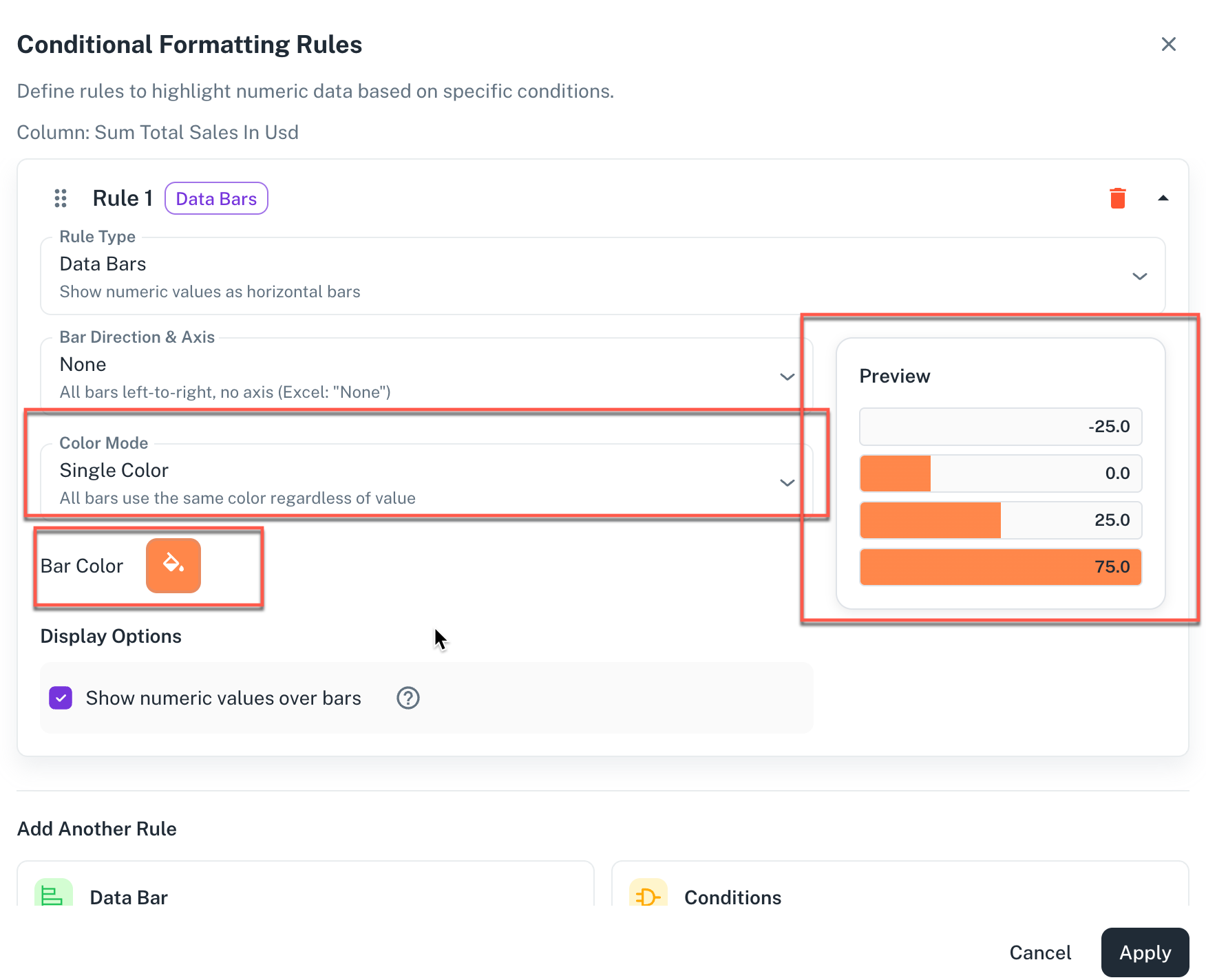
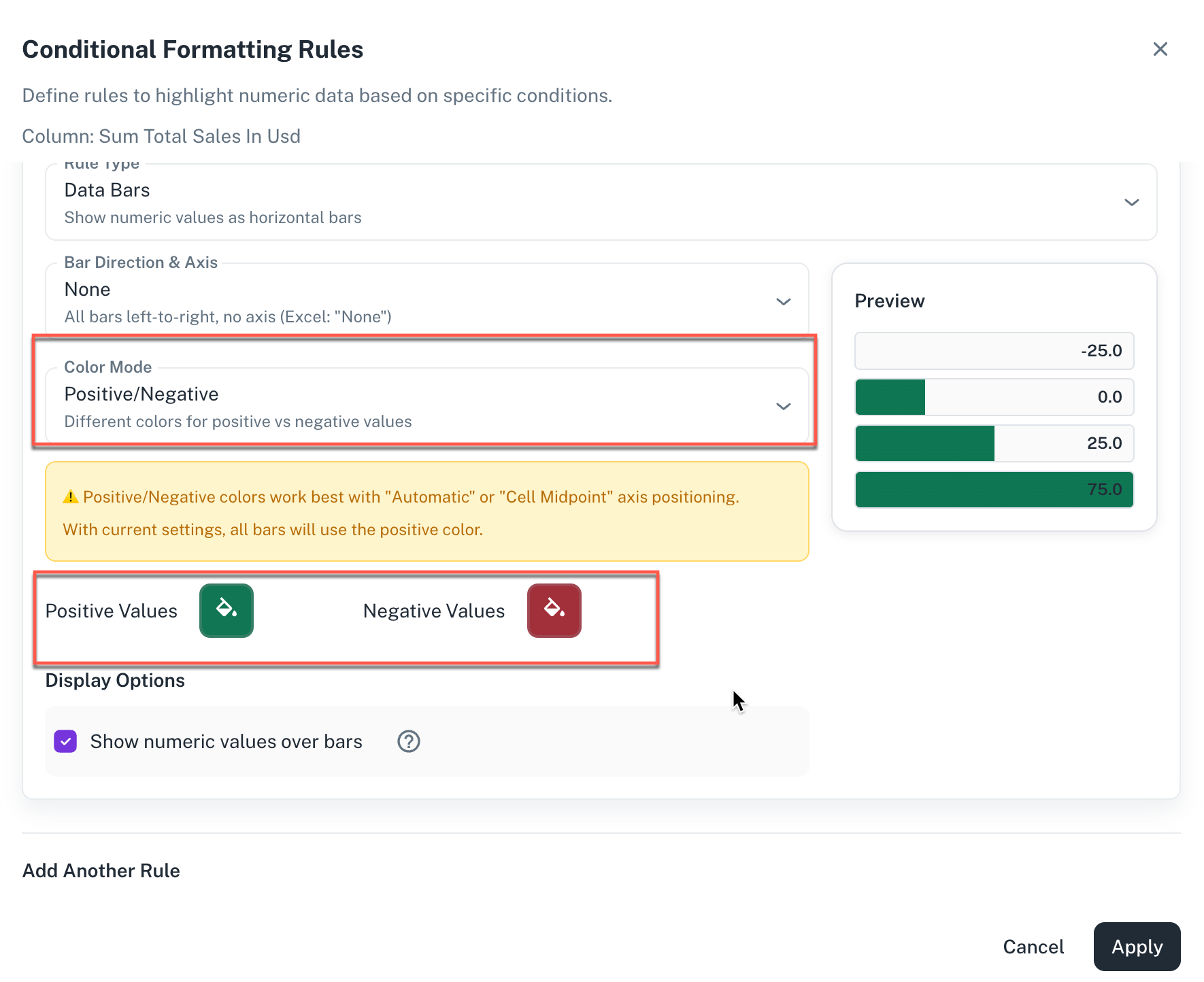
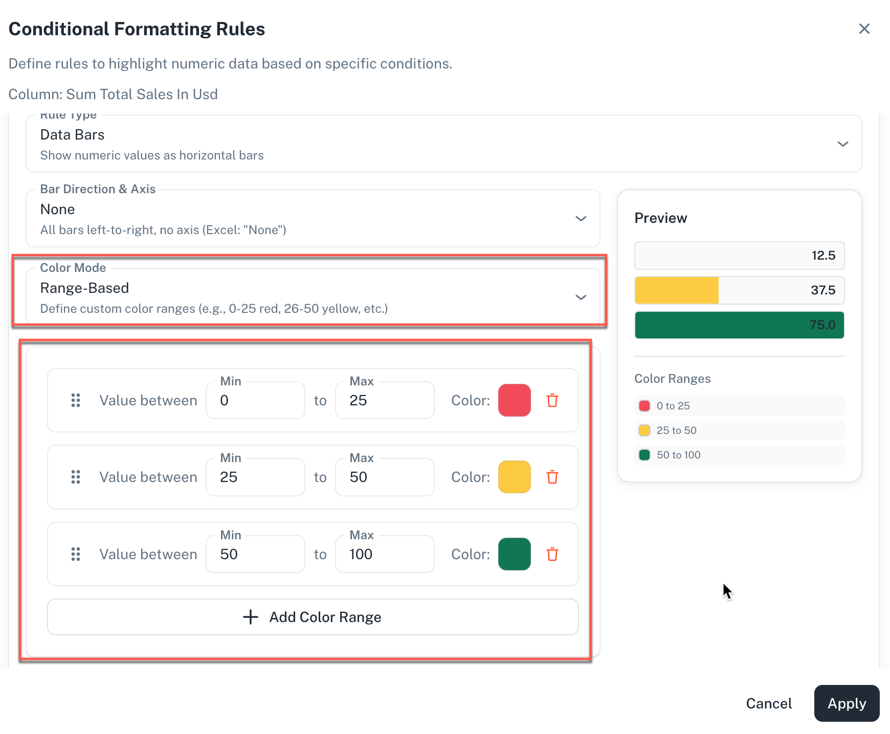
   • Color Mode: Choose any of the following:

     • Single Color: All the bars use the same color regardless of the value. Click the Bar color to set the single color.

       

     • Positive/Negative: Different colors are used for positive and negative values. You can further set the positive and negatie colors.

       

     • Range Based: Define custom color ranges. For example: 0-25 red, 25-50 yellow, and 50-100 green.

       

   • Show numeric values over bars: Check this option to show the actual numbers on top of the bars.

6. Optionally, you can add rules or conditions.

7. Click Apply and in the slide-out menu, click Apply. The conditional formatting gets applied with the conditions or rules set are met.

How to view and manage conditional formatting?

After applying your rules, you can see the formatting in the columns when the conditions or rules that you had set are fulfilled.

• Cross-visualization support: Conditional formatting applied to a value column will be retained when you switch the visualization type, such as from a table to a pivot table. This ensures consistency across your reports.
• Managing multiple rules: You can apply multiple rules to the same column. The system checks the rules in the order they are listed. If a cell meets the criteria of the first rule, that formatting is applied, and the other rules for that cell are ignored.