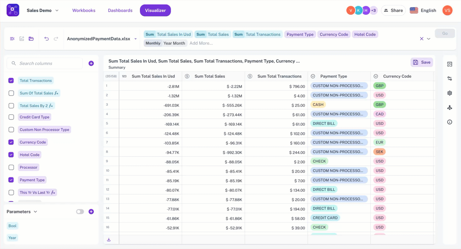
Conditional Formatting for Tables and Pivot Tables
Enhance your data analysis with the new conditional formatting feature for tables and pivot tables. You can now define custom rules and dynamically color-code cells based on their values, allowing for quick visual identification of key data points that meet specific thresholds or criteria.
For example, you can highlight revenue cells in green if they exceed $10,000, yellow if they fall between $5,000 and $10,000, and red if they are below $5,000.
This feature is available only for Table and Pivot table widgets.
The conditions are defined based on the following values:
-
Thresholds: Set rules based on whether a value is greater than, less than, greater than or equal to, or less than or equal to a specific number (e.g., color all values over 10,000,000 green).
-
Ranges: Define a spectrum of colors for values falling within a specified minimum and maximum (e.g., shade values between X and Y in a gradient of yellow).
Customize formatting styles: Choose to alter the text color and/or the background color of the cells to effectively draw attention to specific data points.
Multiple Conditions per column: Apply several conditional formatting rules to a single column, allowing for nuanced visual analysis.